Galaxy NGS 101
This page is designed to serve as a comprehensive resource describing manipulation and analysis of NGS data. While it is designed to highlight the utility of Galaxy it will also provide information that is broadly applicable and can be used for teaching of big data biology. It is accompanied by a collection of screencasts.
Overview of NGS technologies
This section contains quick explanations and important references for major sequencing technologies used today. It is regularly refreshed and kept up-to-date.
Publications:
- Description of 454 process - Margulies et al. (2005)
- Overview of pyrosequencing methodology - Ronaghi (2001)
- History of pyrosequencing - Pål Nyrén (2007)
- Properties of 454 data - Balzer et al. (2010)
- Errors in 454 data - Huse et al. (2007)
Publications:
- Human genome sequencing on Illumina - Bentley et al. (2008)
- Illumina pitfalls - Kircher et al. (2011)
- Data quality 1 - Minoche et al. (2011)
- Data quality 2 - Nakamura et al. (2010)
Publications:
- Semiconmductor non-optical sequencing - Rothberg et al. (2011)
- Ion Torrent, Illumina, PacBio comparison - Quail et al. (2011)
- Improving Ion Torrent Error Rates - Golar and Medvedev (2013)
Publications:
- Single Molecule Analaysis at High Concentration - Levene et al. (2003)
- ZMW nanostructures - Korlach et al. (2008)
- Real Time Sequencing with PacBio - Eid et al. (2009)
- Modification detection with PacBio - Flusberg et al. (2010)
- Error correction of PacBio reads - Koren et al. (2012)
- Transcriptome with PacBio - Taligner et al. (2014)
- Resolving complex regions with PacBio - Chaisson et al. (2015)
Getting data in
You can data in Galaxy using one of five ways:
- From your local computer | Video NGS101-1 | This works best for small files.
- From FTP | Video NGS101-2 | The FTP mechanism allows transferring large collections of files. This is the preferred mechanism for uploading large datasets to Galaxy.
- From the web | Video NGS101-3 | Upload from the web works when URL (addresses) of data files are known
- From EBI short read archive | Video NGS101-4 | This is the best way to upload published datasets deposited to EBI SRA. The problem is that not all datasets are available from EBI. #5 below explain how to deal with NCBI SRA datasets
- Fooling NCBI SRA to produce fastq on the fly | Video NGS101-5 | A tricky but reliable way to get few datasets from NCBI SRA
Fastq manipulation and quality control
Video NGS101-6 | Galaxy History
One of the first steps in the analysis of NGS data is seeing how good the data actually is. FastQC is a fantastic tool allowing you to gauge the quality of fastq datasets (and deciding whether to blame or not to blame whoever has done sequencing for you).
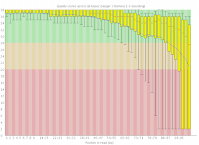
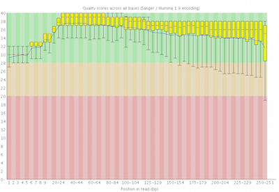
Here you can see FastQC base quality reports (the tools gives you many other types of data) for two datasets: A and B. The A dataset has long reads (250 bp) and very good quality profile with no qualities dropping below phred value of 30. The B dataset is significantly worse with ends of the reads dipping below phred score of 20. The B reads may need to be trimmed for further processing.
Fastq has many faces
Fastq is not a very well defined format. In the beginning various manufacturers of sequencing instruments were free to interpret fastq as they saw fit, resulting in a multitude of fastq flavors. This variation stemmed primarily from different ways of encoding quality values as described here. Today, fastq sanger version of the format is considered to be the standard form of fastq. Galaxy is using fastq sanger as the only legitimate input for downstream processing tools and provides a number of utilities for converting fastq files into this form (see NGS: QC and manipulation section of Galaxy tools).
Mapping your data
Mapping of NGS reads against reference sequences is one of the key steps of the analysis. Basic understanding of how mapping works is just as important as knowing the effects of temperature and magnesium concentration on PCR reaction performance. Below is a list of key publications highlighting basic principles of current mapping tools:
- How to map billions of short reads onto genomes? - Trapnell & Salzberg (2009)
- Bowtie 1 - Langmead et al. (2009)
- Bowtie 2 - Langmead and Salzberg (2012)
- BWA - Li and Durbin (2009)
- BWA - Li and Durbin (2010)
- BWA-MEM - Li (2013)
- Bioinformatics Algorithms - Compeau and Pevzner (2014)
Mapping against a pre-computed genome index
Video NGS101-7 | Galaxy history
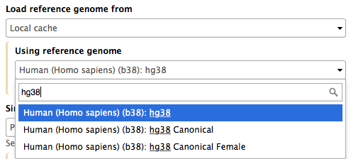
Mappers usually compare reads against a reference sequence that has been transformed into a highly accessible data structure called genome index. Such indices should be generated before mapping begins. Galaxy instances typically store indices for a number of publicly available genome builds. For example, the image on the right shows indices for hg38 version of the human genome. You can see that there are actually three choices: (1) hg38, (2) hg38 canonical and (3) hg38 canonical female. The hg38 contains all chromosomes as well as all unplaced contigs. The hg38 canonical does not contain unplaced sequences and only consists of chromosomes 1 through 22, X, Y, and mitochondria. The hg38 canonical female contains everything from the canonical set with the exception of chromosome Y.
What if pre-computed index does not exist?
Video NGS101-8 | Galaxy history
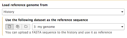
If Galaxy does not have a genome you need to map against, you can upload your genome sequence as a FASTA file and use it in the mapper directly as shown on the right ("Load reference genome" is set to History). In this case Galaxy will first create an index from this dataset and then run mapping analysis against it.
Understanding and manipulating SAM/BAM datasets
The SAM/BAM format is an accepted standard for storing aligned reads (it can also store unaligned reads and some mappers such as BWA are accepting unaligned BAM as input). The binary form of the format (BAM) is compact and can be rapidly searched (if indexed). In Galaxy BAM datasets are always indexed (accompanies by a .bai file) and sorted in coordinate order.
Read groups
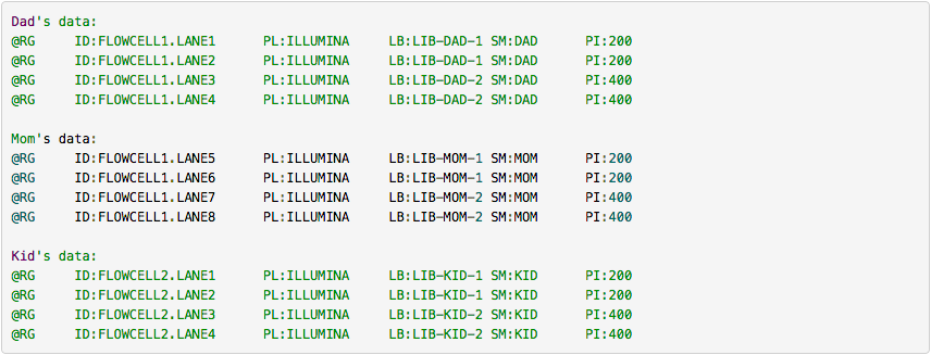
One of the key features of SAM/BAM format is the ability to label individual reads with readgroup tags. This allows pooling results of multiple experiments into a single BAM dataset. This significantly simplifies downstream logistics: instead of dealing with multiple datasets one can handle just one. Many downstream analysis tools such as variant callers are designed to recognize readgroup data and output results on per-readgroup basis.
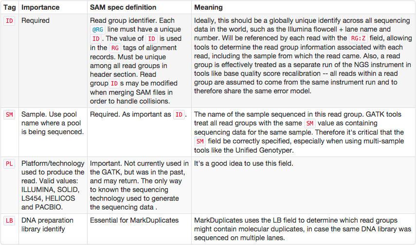
One of the best descriptions of BAM readgroups is on GATK support site. We have gratefully stolen two tables describing the most important readgroup tags -- ID, SM, LB, and PL -- from GATK forum and provide them here.
The following screencast shows how to add readgroups to a BAM dataset in Galaxy using Picard's AddOrReplaceReadGroups tool.
BAM manipulation
Video NGS101-9 = Tweaking BAM | Galaxy history
We support four toolsets for processing of SAM/BAM datasets:
- DeepTools - a suite of user-friendly tools for the visualization, quality control and normalization of data from deep-sequencing DNA sequencing experiments.
- SAMtools - various utilities for manipulating alignments in the SAM/BAM format, including sorting, merging, indexing and generating alignments in a per-position format.
- BAMtools - a toolkit for reading, writing, and manipulating BAM (genome alignment) files.
- Picard - a set of Java tools for manipulating high-throughput sequencing data (HTS) data and formats.
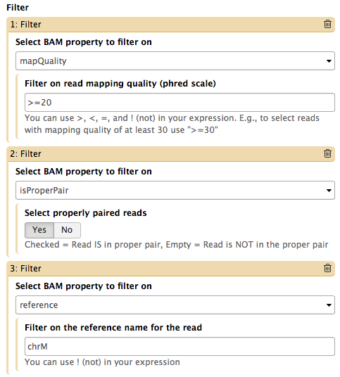
The Screencast NGS101-9 highlight de-duplication, filtering, and cleaning of a BAM dataset using BAMtools and Picard tools.
Finding variants
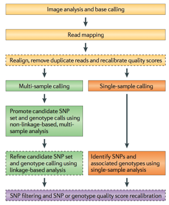
Because of the efforts such as the 1000 Genomes Project, variant calling is one of the most developed areas of NGS analysis. Still, if you are interested in reliable finding of genetic variants it pays to understand how these approaches work. Below we provide a sampler of key publications on the subject.
- Nielsen et al. 2011 - Genotype and SNP calling from NGS data
- Frazer et al. 2009 - Human genetic variation and its contribution to complex traits
- Bamshad et al. 2011 - Exome sequencing as a tool for Mendelian disease gene discover
- Cooper and Shendure 2011 - Finding disease-causal variants in a wealth of genomic data
- Garrison and Marth 2012 - Haplotype-based variant detection from short-read sequencing
- Paila et al. 2013 - GEMINI: Integrative Exploration of Genetic Variation and Genome Annotations
Non-diploid variant calling
Video NGS101-10 = Non-diploid variant calling with NVC | Galaxy history
Video NGS101-11 = Non-diploid variant calling with FreeBayes | Galaxy history
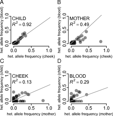
The 1000 Genomes was focused on surveying the genetic diversity of humans - a diploid organism. Yet the majority of life on Earth is non-diploid and represented by prokaryotes, viruses and their derivatives such as our own mitochondria. In non-diploid organisms allele frequencies can range anywhere between 0 and 100% and there could be multiple (not just two) alleles per locus. The main challenge associated with non-diploid variant calling is the ability to distinguish between sequencing noise (abundant in all NGS platforms) and true low frequency variants. Some of the early attempts to do this well have been accomplished on human mitochondrial DNA although the same approaches will work equally good on viral and bacterial genomes:
- Rebolledo-Jaramillo et al. 2014 - Maternal age effect and severe germ-line bottleneck in the inheritance of human mitochondrial DNA
- Li et al. 2015 - Extensive tissue-related and allele-related mtDNA heteroplasmy suggests positive selection for somatic mutations
Visualizing multiple datasets in Integrated Genome Viewer (IGV)
Video NGS101-12 = Displaying multiple tracks in IGV
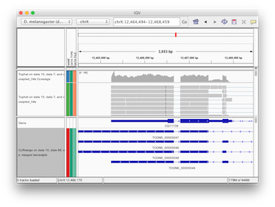
Galaxy has a number of display applications allowing visualization of various datasets. IGV (integrative genome viewer) is one of the most versatile applications for looking at positional genomic data. In Galaxy you can view Interval, BED, BAM, and VCF datasets in IGV. The screencast shows how to do this.
Reference-based RNA-seq
Video NGS101-14 = Mapping reads with TopHat
Video NGS101-15 = Reconstructing transcripts with CuffLinks
Video NGS101-16 = Processing CuffDiff output with Cummerbund
Galaxy RNA-seq workshop slides
Galaxy history containing the entire analysis
There is a number of established strategies for performing RNA-seq analyses when the reference genome of an organism in question is available (for a recent comprehensive comparison see an assement of spliced aligners and an evaluation of transcript reconstruction methods).
The public Galaxy instance at http://usegalaxy.org has been successfully employing Tuxedo suite of tools for references-based RNA-seq originating from Computational Biology and Genomics Lab at Johns Hopkins. However, there are also great resources such as Oqtans developed at the Memorial Sloan-Kettering Cancer Center and others. Below are some of the key publications on the reference-based RNA-seq:
- TopHat: discovering splice junctions with RNA-Seq - Trapnell et al. (2009)
- Transcript assembly and quantification by RNA-Seq reveals unannotated transcripts and isoform switching during cell differentiation - Trapnell et al. (2010)
- Reference guided transcriptome analaysis with TopHat and CuffLinks - Trapnell et al. (2012)
- TopHat2: accurate alignment of transcriptomes in the presence of insertions, deletions and gene fusions - Kim et al. 2013
- Improving RNA-Seq expression estimates by correcting for fragment bias - Roberts et al. (2013)
- Systematic evaluation of spliced alignment programs for RNA-seq data - Engström et al. (2013)
- Assessment of transcript reconstruction methods for RNA-seq - Steijger et al. (2013)
- Oqtans: The RNA-seq Workbench in the Cloud for Complete and Reproducible Quantitative Transcriptome Analysis - Sreedharan et al. (2014)
- HISAT: a fast spliced aligner with low memory requirements - Kim et al. (2015)
- StringTie enables improved reconstruction of a transcriptome from RNA-seq reads - Petrea et al. (2015)
Getting data and mapping to the reference
Video NGS101-14 = Mapping reads with TopHat
In this tutorial we are repeating the steps of a typical RNA-seq analysis described by Trapnell et al. (2012) with one little exception: we have created a set of smaller input files to make this tutorial faster. These data can be accessed here as a Galaxy history. Simply click import history and use it as a starting point of your analysis.
This analysis begins by uploading an annotation file from the UCSC Table Browser and using it as a set of reference gene annotations. The data corresponds to two experimental conditions - Condition 1 and Condition 2 - each containing three replicates. In turn each replicate was sequenced as a mate-pair library and so has two associated datasets: forward and reverse. Thus (2 conditions) x (3 replicates) x (forward and reverse reads) = 2 x 3 x 2 = 12 datasets. We begin by using new Galaxy functionality - dataset collections - to bundle datasets into two collections: one corresponding to condition 1 and the other to condition 2. We then map the reads in each collection against dm3 version of Drosophila melanogaster genome using TopHat2. This generates (among other outputs) BAM outputs containing mapped reads.
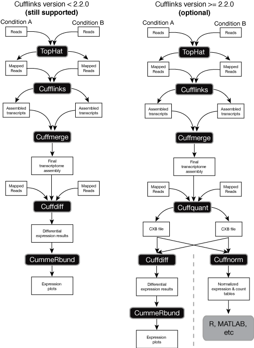
Reconstructing transcripts
Video NGS101-15 = Reconstructing transcripts with CuffLinks
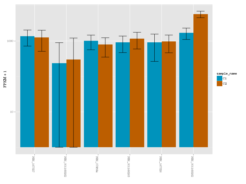
a gene in conditions 1 (blue) and 2 (brown)
Reads mapped by TopHat are then used as input to CuffLinks - a tool that performs transcript reconstruction and quantification. This is done individually for every replicate (although because our data is bundled in collections this is a painless exercise). Once transcript reconstruction is finished we combine transcript model from all replicates and conditions into a single transcriptome using CuffMerge. Finally, we perform differential expression analysis with CuffDiff using the combined transcriptome and read mapping data.
Finding differentially expressed transcripts
Video NGS101-16 = Processing CuffDiff output with Cummerbund
Galaxy version of CuffDiff used in the previous step produces a database. Using Extract CuffDiff data and Filter tools we retrieve a list of differentially expressed genes and visualize expression level for transcripts of one such gene using CummerBund.
HISAT and StringTie
The mapping and transcript reconstruction steps of the reference-based RNA-seq analysis will soon be complemented with the addition of HISAT and StringTie tools. Stay tuned for updates.
What is coming next?
- RNA secondary structure prediction
- Reference-free RNA-seq with Trinity
- DNA/Protein Interactions
- 16S & shotgun metagenomics
- Visualization of NGS data